GokuMohandas/monitoring-ml

GokuMohandas/monitoring-ml — an AI tool — sits at 105 GitHub stars in the AI Tools space. Learn how to monitor ML systems to identify and mitigate sources of drift before model performance decay.
Snapshot summary built from the project's own GitHub metadata — there's no written TopGit review yet. The page will update automatically when a full review is published.
TopGit writes full reviews for the most-starred, most-requested repositories. This page is a snapshot until then — see the READ ME tab for the original README in full.
Snapshot
Top contributors
Show top contributors
Monitoring ML
Learn how to monitor ML systems to identify and address sources of drift before model performance decay.


👉 This repository contains the interactive notebook that complements the monitoring lesson, which is a part of the MLOps course. If you haven't already, be sure to check out the lesson because all the concepts are covered extensively and tied to software engineering best practices for building ML systems.



- Performance
- Drift
- Data drift
- Target drift
- Concept drift
- Locating drift
- Measuring drift
- Expectations
- Univariate
- Multivariate
- Online
Performance
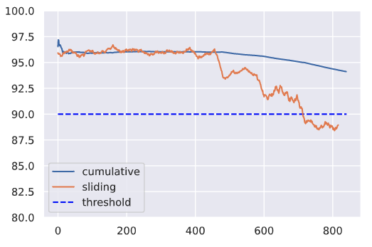
A key aspect of monitoring ML systems involves monitoring the actual performance of our deployed models. These could be quantitative evaluation metrics that we used during model evaluation (accuracy, precision, f1, etc.) but also key business metrics that the model influences (ROI, click rate, etc.). And it's usually never enough to just analyze the cumulative performance metrics across the entire span of time since the model has been deployed. Instead, we should also inspect performance across a period of time that's significant for our application (ex. daily). These sliding metrics might be more indicative of our system's health and we might be able to identify issues faster by not obscuring them with historical data.
import matplotlib.pyplot as plt
import numpy as np
import seaborn as sns
sns.set_theme()
# Generate data
hourly_f1 = list(np.random.randint(low=94, high=98, size=24*20)) + \
            list(np.random.randint(low=92, high=96, size=24*5)) + \
            list(np.random.randint(low=88, high=96, size=24*5)) + \
            list(np.random.randint(low=86, high=92, size=24*5))
# Cumulative f1
cumulative_f1 = [np.mean(hourly_f1[:n]) for n in range(1, len(hourly_f1)+1)]
print (f"Average cumulative f1 on the last day: {np.mean(cumulative_f1[-24:]):.1f}")
Average cumulative f1 on the last day: 93.7
# Sliding f1
window_size = 24
sliding_f1 = np.convolve(hourly_f1, np.ones(window_size)/window_size, mode="valid")
print (f"Average sliding f1 on the last day: {np.mean(sliding_f1[-24:]):.1f}")
Average sliding f1 on the last day: 88.6
plt.ylim([80, 100])
plt.hlines(y=90, xmin=0, xmax=len(hourly_f1), colors="blue", linestyles="dashed", label="threshold")
plt.plot(cumulative_f1, label="cumulative")
plt.plot(sliding_f1, label="sliding")
plt.legend()
Drift
We need to first understand the different types of issues that can cause our model's performance to decay (model drift). The best way to do this is to look at all the moving pieces of what we're trying to model and how each one can experience drift.
| Entity | Description | Drift |
|---|---|---|
| $X$ | inputs (features) | data drift $\rightarrow P(X) \neq P_{ref}(X)$ |
| $y$ | outputs (ground-truth) | target drift $\rightarrow P(y) \neq P_{ref}(y)$ |
| $P(y \vert X)$ | actual relationship between $X$ and $y$ | concept drift $\rightarrow P(y \vert X) \neq P_{ref}(y \vert X)$ |
Data drift
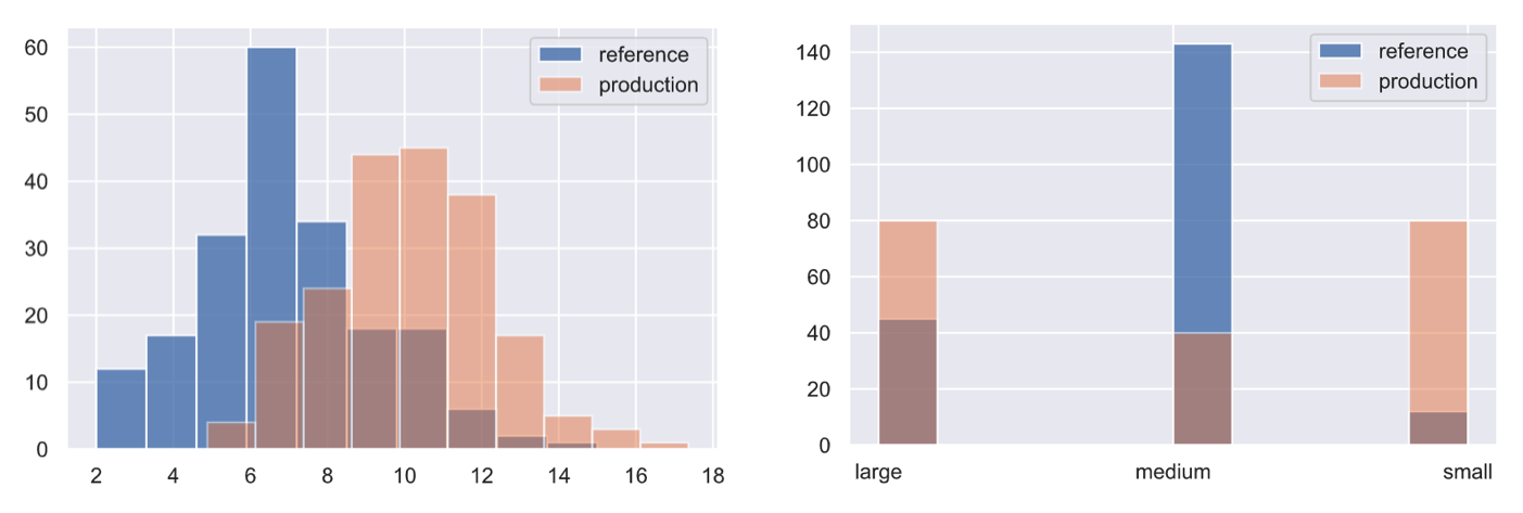
Data drift, also known as feature drift or covariate shift, occurs when the distribution of the production data is different from the training data. The model is not equipped to deal with this drift in the feature space and so, it's predictions may not be reliable. The actual cause of drift can be attributed to natural changes in the real-world but also to systemic issues such as missing data, pipeline errors, schema changes, etc. It's important to inspect the drifted data and trace it back along it's pipeline to identify when and where the drift was introduced.
Target drift
Besides just the input data changing, as with data drift, we can also experience drift in our outcomes. This can be a shift in the distributions but also the removal or addition of new classes with categorical tasks. Though retraining can mitigate the performance decay caused target drift, it can often be avoided with proper inter-pipeline communication about new classes, schema changes, etc.
Concept drift
Besides the input and output data drifting, we can have the actual relationship between them drift as well. This concept drift renders our model ineffective because the patterns it learned to map between the original inputs and outputs are no longer relevant. Concept drift can be something that occurs in various patterns:
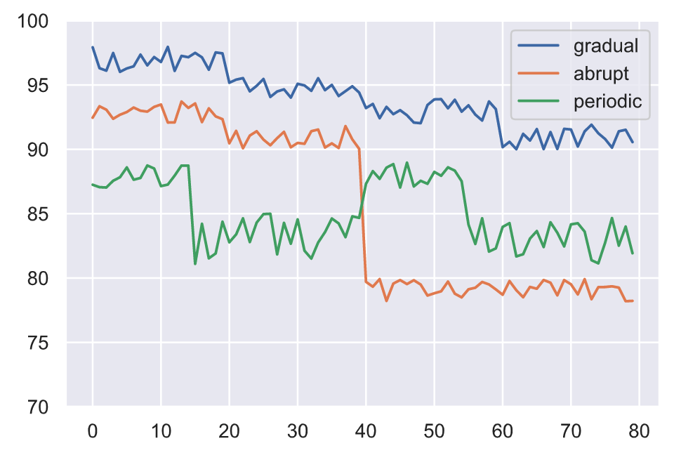
- gradually over a period of time
- abruptly as a result of an external event
- periodically as a result of recurring events
All the different types of drift we discussed can can occur simultaneously which can complicated identifying the sources of drift.
Locating drift
Now that we've identified the different types of drift, we need to learn how to locate and how often to measure it. Here are the constraints we need to consider:
- reference window: the set of points to compare production data distributions with to identify drift.
- test window: the set of points to compare with the reference window to determine if drift has occurred.
Since we're dealing with online drift detection (ie. detecting drift in live production data as opposed to past batch data), we can employ either a fixed or sliding window approach to identify our set of points for comparison. Typically, the reference window is a fixed, recent subset of the training data while the test window slides over time.
Measuring drift
Once we have the window of points we wish to compare, we need to know how to compare them.
import great_expectations as ge
import json
import pandas as pd
from urllib.request import urlopen
# Load labeled projects
projects = pd.read_csv("https://raw.githubusercontent.com/GokuMohandas/Made-With-ML/main/datasets/projects.csv")
tags = pd.read_csv("https://raw.githubusercontent.com/GokuMohandas/Made-With-ML/main/datasets/tags.csv")
df = ge.dataset.PandasDataset(pd.merge(projects, tags, on="id"))
df["text"] = df.title + " " + df.description
df.drop(["title", "description"], axis=1, inplace=True)
df.head(5)
| id | created_on | tag | text | |
|---|---|---|---|---|
| 0 | 6 | 2020-02-20 06:43:18 | computer-vision | Comparison between YOLO and RCNN on real world... |
| 1 | 7 | 2020-02-20 06:47:21 | computer-vision | Show, Infer & Tell: Contextual Inference for C... |
| 2 | 9 | 2020-02-24 16:24:45 | graph-learning | Awesome Graph Classification A collection of i... |
| 3 | 15 | 2020-02-28 23:55:26 | reinforcement-learning | Awesome Monte Carlo Tree Search A curated list... |
| 4 | 19 | 2020-03-03 13:54:31 | graph-learning | Diffusion to Vector Reference implementation o... |
Expectations
The first line of measurement can be rule-based such as validating expectations around missing values, data types, value ranges, etc. as we did in our data testing lesson. These can be done with or without a reference window and using the mostly argument for some level of tolerance.
# Simulated production data
prod_df = ge.dataset.PandasDataset([{"text": "hello"}, {"text": 0}, {"text": "world"}])
# Expectation suite
df.expect_column_values_to_not_be_null(column="text")
df.expect_column_values_to_be_of_type(column="text", type_="str")
expectation_suite = df.get_expectation_suite()
# Validate reference data
df.validate(expectation_suite=expectation_suite, only_return_failures=True)["statistics"]
{"evaluated_expectations": 2,
 "success_percent": 100.0,
 "successful_expectations": 2,
 "unsuccessful_expectations": 0}
# Validate production data
prod_df.validate(expectation_suite=expectation_suite, only_return_failures=True)["statistics"]
{"evaluated_expectations": 2,
 "success_percent": 50.0,
 "successful_expectations": 1,
 "unsuccessful_expectations": 1}
Once we've validated our rule-based expectations, we need to quantitatively measure drift across the different features in our data.
Univariate
Our task may involve univariate (1D) features that we will want to monitor. While there are many types of hypothesis tests we can use, a popular option is the Kolmogorov-Smirnov (KS) test.
Kolmogorov-Smirnov (KS) test
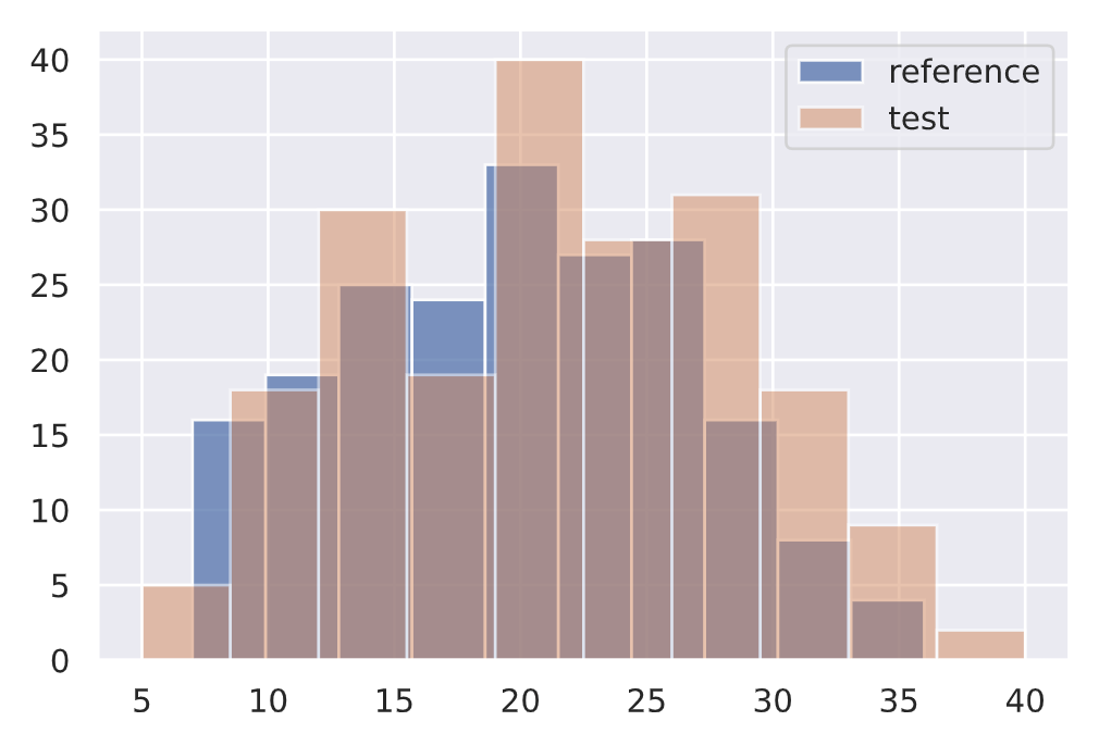
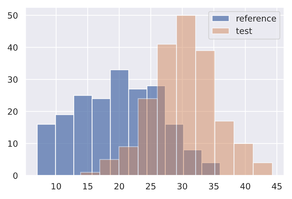
The KS test determines the maximum distance between two distribution's cumulative density functions. Here, we'll measure if there is any drift on the size of our input text feature between two different data subsets.
from alibi_detect.cd import KSDrift
# Reference
df["num_tokens"] = df.text.apply(lambda x: len(x.split(" ")))
ref = df["num_tokens"][0:200].to_numpy()
plt.hist(ref, alpha=0.75, label="reference")
plt.legend()
plt.show()
# Initialize drift detector
length_drift_detector = KSDrift(ref, p_val=0.01)
# No drift
no_drift = df["num_tokens"][200:400].to_numpy()
plt.hist(ref, alpha=0.75, label="reference")
plt.hist(no_drift, alpha=0.5, label="test")
plt.legend()
plt.show()
length_drift_detector.predict(no_drift, return_p_val=True, return_distance=True)
{"data": {"distance": array([0.09], dtype=float32),
  "is_drift": 0,
  "p_val": array([0.3927307], dtype=float32),
  "threshold": 0.01},
 "meta": {"data_type": None,
  "detector_type": "offline",
  "name": "KSDrift",
  "version": "0.9.1"}}
↓ p-value = ↑ confident that the distributions are different.
# Drift
drift = np.random.normal(30, 5, len(ref))
plt.hist(ref, alpha=0.75, label="reference")
plt.hist(drift, alpha=0.5, label="test")
plt.legend()
plt.show()
length_drift_detector.predict(drift, return_p_val=True, return_distance=True)
{"data": {"distance": array([0.63], dtype=float32),
  "is_drift": 1,
  "p_val": array([6.7101775e-35], dtype=float32),
  "threshold": 0.01},
 "meta": {"data_type": None,
  "detector_type": "offline",
  "name": "KSDrift",
  "version": "0.9.1"}}
Chi-squared test
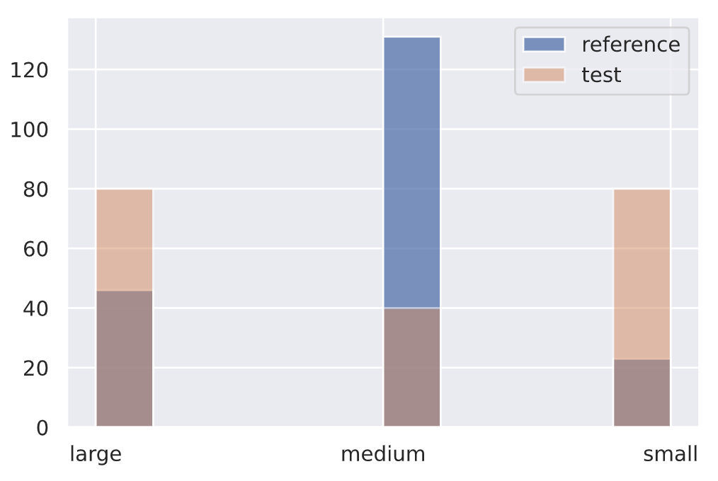
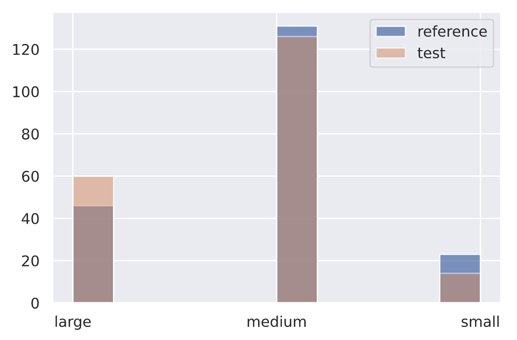
Similarly, for categorical data (input features, targets, etc.), we can apply the Pearson's chi-squared test to determine if a frequency of events in production is consistent with a reference distribution.
We're creating a categorical variable for the # of tokens in our text feature but we could very very apply it to the tag distribution itself, individual tags (binary), slices of tags, etc.
from alibi_detect.cd import ChiSquareDrift
# Reference
df.token_count = df.num_tokens.apply(lambda x: "small" if x <= 10 else ("medium" if x <=25 else "large"))
ref = df.token_count[0:200].to_numpy()
plt.hist(ref, alpha=0.75, label="reference")
plt.legend()
# Initialize drift detector
target_drift_detector = ChiSquareDrift(ref, p_val=0.01)
# No drift
no_drift = df.token_count[200:400].to_numpy()
plt.hist(ref, alpha=0.75, label="reference")
plt.hist(no_drift, alpha=0.5, label="test")
plt.legend()
plt.show()
target_drift_detector.predict(no_drift, return_p_val=True, return_distance=True)
{"data": {"distance": array([4.135522], dtype=float32),
  "is_drift": 0,
  "p_val": array([0.12646863], dtype=float32),
  "threshold": 0.01},
 "meta": {"data_type": None,
  "detector_type": "offline",
  "name": "ChiSquareDrift",
  "version": "0.9.1"}}
# Drift
drift = np.array(["small"]*80 + ["medium"]*40 + ["large"]*80)
plt.hist(ref, alpha=0.75, label="reference")
plt.hist(drift, alpha=0.5, label="test")
plt.legend()
plt.show()
target_drift_detector.predict(drift, return_p_val=True, return_distance=True)
{"data": {"is_drift": 1,
  "distance": array([118.03355], dtype=float32),
  "p_val": array([2.3406739e-26], dtype=float32),
  "threshold": 0.01},
 "meta": {"name": "ChiSquareDrift",
  "detector_type": "offline",
  "data_type": None}}
Multivariate
As we can see, measuring drift is fairly straightforward for univariate data but difficult for multivariate data. We'll summarize the reduce and measure approach outlined in the following paper: Failing Loudly: An Empirical Study of Methods for Detecting Dataset Shift.

Be sure to refer to our embeddings and transformers lessons to learn more about these topics. But note that detecting drift on multivariate text embeddings is still quite difficult so it's typically more common to use these methods applied to tabular features or images.
We'll start by loading the tokenizer from a pretrained model.
from transformers import AutoTokenizer
model_name = "allenai/scibert_scivocab_uncased"
tokenizer = AutoTokenizer.from_pretrained(model_name)
vocab_size = len(tokenizer)
print (vocab_size)
31090
# Tokenize inputs
encoded_input = tokenizer(df.text.tolist(), return_tensors="pt", padding=True)
ids = encoded_input["input_ids"]
masks = encoded_input["attention_mask"]
# Decode
print (f"{ids[0]}\n{tokenizer.decode(ids[0])}")
tensor([  102,  2029,   467,  1778,   609,   137,  6446,  4857,   191,  1332,
         2399, 13572, 19125,  1983,   147,  1954,   165,  6240,   205,   185,
          300,  3717,  7434,  1262,   121,   537,   201,   137,  1040,   111,
          545,   121,  4714,   205,   103,     0,     0,     0,     0,     0,
            0,     0,     0,     0,     0,     0,     0,     0,     0,     0,
            0,     0,     0,     0,     0,     0,     0,     0,     0,     0,
            0])
[CLS] comparison between yolo and rcnn on real world videos bringing theory to experiment is cool. we can easily train models in colab and find the results in minutes. [SEP] [PAD] [PAD] ...
# Sub-word tokens
print (tokenizer.convert_ids_to_tokens(ids=ids[0]))
['[CLS]', 'comparison', 'between', 'yo', '##lo', 'and', 'rc', '##nn', 'on', 'real', 'world', 'videos', 'bringing', 'theory', 'to', 'experiment', 'is', 'cool', '.', 'we', 'can', 'easily', 'train', 'models', 'in', 'col', '##ab', 'and', 'find', 'the', 'results', 'in', 'minutes', '.', '[SEP]', '[PAD]', '[PAD]', ...]
Next, we'll load the pretrained model's weights and use the TransformerEmbedding object to extract the embeddings from the hidden state (averaged across tokens).
from alibi_detect.models.pytorch import TransformerEmbedding
# Embedding layer
emb_type = "hidden_state"
layers = [-x for x in range(1, 9)]  # last 8 layers
embedding_layer = TransformerEmbedding(model_name, emb_type, layers)
# Embedding dimension
embedding_dim = embedding_layer.model.embeddings.word_embeddings.embedding_dim
embedding_dim
768
Dimensionality reduction
Now we need to use a dimensionality reduction method to reduce our representations dimensions into something more manageable (ex. 32 dim) so we can run our two-sample tests on to detect drift. Popular options include:
- Principle component analysis (PCA): orthogonal transformations that preserve the variability of the dataset.
- Autoencoders (AE): networks that consume the inputs and attempt to reconstruct it from an lower dimensional space while minimizing the error. These can either be trained or untrained (the Failing loudly paper recommends untrained).
- Black box shift detectors (BBSD): the actual model trained on the training data can be used as a dimensionality reducer. We can either use the softmax outputs (multivariate) or the actual predictions (univariate).
import torch
import torch.nn as nn
# Device
device = torch.device("cuda" if torch.cuda.is_available() else "cpu")
print(device)
cuda
# Untrained autoencoder (UAE) reducer
encoder_dim = 32
reducer = nn.Sequential(
    embedding_layer,
    nn.Linear(embedding_dim, 256),
    nn.ReLU(),
    nn.Linear(256, encoder_dim)
).to(device).eval()
We can wrap all of the operations above into one preprocessing function that will consume input text and produce the reduced representation.
from alibi_detect.cd.pytorch import preprocess_drift
from functools import partial
# Preprocessing with the reducer
max_len = 100
batch_size = 32
preprocess_fn = partial(preprocess_drift, model=reducer, tokenizer=tokenizer,
                        max_len=max_len, batch_size=batch_size, device=device)
Maximum Mean Discrepancy (MMD)
After applying dimensionality reduction techniques on our multivariate data, we can use different statistical tests to calculate drift. A popular option is Maximum Mean Discrepancy (MMD), a kernel-based approach that determines the distance between two distributions by computing the distance between the mean embeddings of the features from both distributions.
from alibi_detect.cd import MMDDrift
# Initialize drift detector
mmd_drift_detector = MMDDrift(ref, backend="pytorch", p_val=.01, preprocess_fn=preprocess_fn)
# No drift
no_drift = df.text[200:400].to_list()
mmd_drift_detector.predict(no_drift)
{"data": {"distance": 0.0021169185638427734,
  "distance_threshold": 0.0032651424,
  "is_drift": 0,
  "p_val": 0.05999999865889549,
  "threshold": 0.01},
 "meta": {"backend": "pytorch",
  "data_type": None,
  "detector_type": "offline",
  "name": "MMDDriftTorch",
  "version": "0.9.1"}}
# Drift
drift = ["UNK " + text for text in no_drift]
mmd_drift_detector.predict(drift)
{"data": {"distance": 0.014705955982208252,
  "distance_threshold": 0.003908038,
  "is_drift": 1,
  "p_val": 0.0,
  "threshold": 0.01},
 "meta": {"backend": "pytorch",
  "data_type": None,
  "detector_type": "offline",
  "name": "MMDDriftTorch",
  "version": "0.9.1"}}
Online
So far we've applied our drift detection methods on offline data to try and understand what reference window sizes should be, what p-values are appropriate, etc. However, we'll need to apply these methods in the online production setting so that we can catch drift as easy as possible.
Many monitoring libraries and platforms come with online equivalents for their detection methods.
Typically, reference windows are large so that we have a proper benchmark to compare our production data points to. As for the test window, the smaller it is, the more quickly we can catch sudden drift. Whereas, a larger test window will allow us to identify more subtle/gradual drift. So it's best to compose windows of different sizes to regularly monitor.
from alibi_detect.cd import MMDDriftOnline
# Online MMD drift detector
ref = df.text[0:800].to_list()
online_mmd_drift_detector = MMDDriftOnline(
    ref, ert=400, window_size=200, backend="pytorch", preprocess_fn=preprocess_fn)
Generating permutations of kernel matrix..
100%|██████████| 1000/1000 [00:00<00:00, 13784.22it/s]
Computing thresholds: 100%|██████████| 200/200 [00:32<00:00,  6.11it/s]
As data starts to flow in, we can use the detector to predict drift at every point. Our detector should detect drift sooner in our drifter dataset than in our normal data.
def simulate_production(test_window):
    i = 0
    online_mmd_drift_detector.reset()
    for text in test_window:
        result = online_mmd_drift_detector.predict(text)
        is_drift = result["data"]["is_drift"]
        if is_drift:
            break
        else:
            i += 1
    print (f"{i} steps")
# Normal
test_window = df.text[800:]
simulate_production(test_window)
27 steps
# Drift
test_window = "UNK" * len(df.text[800:])
simulate_production(test_window)
11 steps
There are also several considerations around how often to refresh both the reference and test windows. We could base in on the number of new observations or time without drift, etc. We can also adjust the various thresholds (ERT, window size, etc.) based on what we learn about our system through monitoring.
Learn more
While these are the foundational concepts for monitoring ML systems, there are a lot of software best practices for monitoring that we cannot show in an isolated repository. Learn more in our monitoring lesson.
Related repositories
TensorFlow is Google's open-source, end-to-end platform for machine learning, hosted at tensorflow/tensorflow under the Apache-2.0 license. It was originally built within Google Brain's Machine Intelligence team for ML and neural network research, and today it ships stable Python and C++ APIs alongside GPU, CPU-only, and Docker install paths. The README positions it as covering both research work and shipping ML-powered applications.
prompts.chat is the largest open-source prompt library for AI, formerly called Awesome ChatGPT Prompts. It hosts curated prompts in CSV and Markdown, available as a public website, Hugging Face dataset, or self-hosted instance. The project supports multiple LLM providers including ChatGPT, Claude, Gemini, Llama, and Mistral. Self-hosting uses a Next.js setup wizard that configures authentication via GitHub, Google, or Azure AD, with PostgreSQL as the recommended database. CLI access, an MCP server, and a Claude Code plugin extend its reach into developer workflows. The codebase is MIT-licensed while prompt data falls under CC0. Its 166k GitHub stars make it an AI resource on the platform with 166k GitHub stars, and it has been cited by Harvard, Columbia, and Forbes.
prompts.chat is an open-source library of prompts written for AI chat assistants, first released in December 2022 under the name Awesome ChatGPT Prompts. The GitHub project has since grown to 167,080 stars and 21,564 forks, and now distributes prompts through a website, a CSV file, a Markdown file, and a Hugging Face dataset, alongside a self-hosting option, a CLI, an MCP server, and a Claude Code plugin.
Hugging Face Transformers (huggingface/transformers) is a Python library that centralizes model definitions for text, computer vision, audio, video, and multimodal machine learning, covering both inference and training. The README describes it as a pivot point compatible with training frameworks such as Axolotl, DeepSpeed, and PyTorch-Lightning, and inference engines such as vLLM, SGLang, and TGI, with more than 1M+ model checkpoints listed on the Hugging Face Hub.
Quick answers
Does GokuMohandas/monitoring-ml have a project website?
No homepage URL was recorded for GokuMohandas/monitoring-ml in TopGit's last sync. The README tab above frequently contains screenshots and demo links, or check the repository description on GitHub.
How does GokuMohandas/monitoring-ml compare to other AI Tools projects?
GokuMohandas/monitoring-ml is tracked by TopGit in the AI Tools category, with 105 GitHub stars and written in Jupyter Notebook. Browse the AI Tools topic page on TopGit to compare it against similar projects by stars and activity.
How many stars does GokuMohandas/monitoring-ml have?
GokuMohandas/monitoring-ml has 105 GitHub stars — refresh the page for the live number, or check github.com/GokuMohandas/monitoring-ml. TopGit mirrors GitHub's count but does not claim minute-by-minute accuracy.
Is GokuMohandas/monitoring-ml open source?
TopGit's metadata for GokuMohandas/monitoring-ml does not record a license. Most public repositories on GitHub ARE open source, but the exact terms vary — verify by opening the LICENSE file directly.
What else is in the AI Tools space?
GokuMohandas/monitoring-ml is tracked by TopGit under the AI Tools category, alongside 4 GitHub-tagged topics. Trending and Topics pages list peer repositories of comparable stars and language.
What is GokuMohandas/monitoring-ml?
GokuMohandas/monitoring-ml (GokuMohandas/monitoring-ml) is a Jupyter Notebook project on GitHub. From the project's own README: Learn how to monitor ML systems to identify and mitigate sources of drift before model performance decay.
Where do I read more about GokuMohandas/monitoring-ml?
This TopGit page is a snapshot — the READ ME tab shows the project's own README content (links stripped, images preserved). The GitHub repository at github.com/GokuMohandas/monitoring-ml is the definitive source.
Read full README in the tab above.
Still deciding about monitoring-ml?
One click hands the question to an AI along with this page — see what it says about monitoring-ml.